06 Compare Models to Select the Best Hyperparameters¶

Published: June, 2024, ATOM DDM Team

Please check out the companion tutorial video:

This tutorial will review AMPL functions for visualizing the results of a hyperparameter search in order to find the optimal hyperparameters for your model.

After performing a hyperparameter search, it is prudent to examine each hyperparameter in order to determine the best combination before training a production model with all of the data. Additionally, it is good to explore multiple performance metrics and visualize the predictions instead of relying solely on metrics.

For the purposes of this tutorial, we simply ran Tutorial 5, “Hyperparameter Optimization”, with different parameters such as those outlined here to get enough models for comparison. Specifically, we created additional NN and XGBoost models as well as using fingerprint and scaffold splits. If you don’t want to run that many models, you can use the result_df saved here: dataset/SLC6A3_models/07_example_pred_df.csv.

In this tutorial, we will focus on these functions:

Import Packages¶

from atomsci.ddm.pipeline import compare_models as cm
from atomsci.ddm.pipeline import hyper_perf_plots as hpp
from atomsci.ddm.pipeline import perf_plots as pp
import pandas as pd
pd.set_option('display.max_columns', None)

# ignore warnings in tutorials
import warnings
warnings.filterwarnings('ignore', category=FutureWarning)
warnings.filterwarnings('ignore', category=RuntimeWarning)

Get Model Results and Filter¶

First we pull the results of the hyperparameter search into a dataframe. In Tutorial 5, “Hyperparameter Optimization”, we used get_filesystem_perf_results() which packs hyperparameters in a dict in the column model_parameters_dict. Here we use the individual hyperparameter columns to create visualizations.

The result_df used here as an example is the result of calling get_filesystem_perf_results() once after training several hundred models with different parameters. These models were all saved in a single folder, but the function works iteratively so it can search an entire directory tree if a parent folder is passed.

# # call the function yourself
# result_df=cm.get_filesystem_perf_results(result_dir='dataset/SLC6A3_models/', pred_type='regression')

# use example results
result_df=pd.read_csv('dataset/SLC6A3_models/07_example_pred_df.csv', index_col=0)

result_df=result_df.sort_values('best_valid_r2_score', ascending=False)
print(result_df.shape)

# show useful columns
result_df[['model_uuid', 'split_uuid', 'best_train_r2_score', 'best_valid_r2_score', 'best_test_r2_score']].head()

(467, 41)

	model_uuid	split_uuid	best_train_r2_score	best_valid_r2_score	best_test_r2_score
310	b24a2887-8eca-43e2-8fc2-3642189d2c94	c35aeaab-910c-4dcf-8f9f-04b55179aa1a	0.776865	0.562091	0.519325
306	9b6c9332-15f3-4f96-9579-bf407d0b69a8	c35aeaab-910c-4dcf-8f9f-04b55179aa1a	0.950677	0.559590	0.480895
291	d8e25713-bf6c-4ba0-917a-69f0ea1472b9	c35aeaab-910c-4dcf-8f9f-04b55179aa1a	0.930726	0.557156	0.497192
334	1a3e4b13-f860-4acf-8300-e2ac5766caa6	c35aeaab-910c-4dcf-8f9f-04b55179aa1a	0.801391	0.556679	0.523567
321	57a62e20-f18e-4afa-8ce2-315f0fcc950a	c35aeaab-910c-4dcf-8f9f-04b55179aa1a	0.780693	0.556103	0.521270

We can look at a brief count of models for important parameters by creating a pivot table. Here we can see ECFP fingerprints and RDKit features and fingerprint and scaffold splitters were used for each model type. A fingerprint splitter provides a more stringent test of model performance by making sure the validation and test compounds are structurally dissimilar to the training set compounds.

# model counts
model_counts=pd.DataFrame(result_df.groupby(['features','splitter','model_type'])['model_uuid'].count()).reset_index()
model_counts=model_counts.pivot(index='model_type',columns=['splitter','features',], values='model_uuid')
model_counts

splitter	fingerprint	scaffold	fingerprint	scaffold
features	ecfp	ecfp	rdkit_raw	rdkit_raw
model_type
NN	26	29	25	96
RF	30	30	30	32
xgboost	47	26	20	76

Often, certain random combinations of hyperparameters result in terribly performing models. Here we will filter those out so they don’t affect the visualization by only keeping models with a validation r2_score of 0.1 or greater.

result_df.best_valid_r2_score.describe()

count    4.670000e+02
mean    -6.111789e+73
std      1.320769e+75
min     -2.854206e+76
25%     -2.751967e-01
50%      2.719028e-01
75%      4.323609e-01
max      5.620908e-01
Name: best_valid_r2_score, dtype: float64

# filter out objectively bad performing models
result_df=result_df[result_df.best_valid_r2_score>0.1]
result_df.shape

(264, 41)

result_df.best_valid_r2_score.describe()

count    264.000000
mean       0.405931
std        0.108515
min        0.110739
25%        0.337459
50%        0.418931
75%        0.484987
max        0.562091
Name: best_valid_r2_score, dtype: float64

After filtering out models with extremely poor metrics, we can see that some combinations don’t work at all, and are completely filtered from the set. For example, decision tree based models using RDKit or ECFP features work very poorly to predict on fingerprint-split models.

#  model counts
model_counts=pd.DataFrame(result_df.groupby(['features','splitter','model_type'])['model_uuid'].count()).reset_index()
model_counts=model_counts.pivot(index='model_type',columns=['splitter','features',], values='model_uuid')
model_counts

splitter	fingerprint	scaffold	fingerprint	scaffold
features	ecfp	ecfp	rdkit_raw	rdkit_raw
model_type
NN	8.0	23.0	11.0	86.0
RF	NaN	30.0	NaN	32.0
xgboost	3.0	21.0	NaN	50.0

Visualize Hyperparameters¶

There are several plotting functions in the hyper_perf_plots module that help visualize the different combinations of features for each type of model.

Examine overall scores¶

plot_train_valid_test_scores() gives a quick snapshot of your overall model performance. You can see if you overfitted and get a sense of whether your partitions are a good representation of future performance. Because the splitter can have a drastic effect on model performance, these plots are also separated by split type.

Here we see a fairly typical pattern where the training set metrics are higher than validation and test partitions. It is good to see that the validation and test scores are similar across many models, indicating that the models should generalize to new data well. For fingerprint splits, we see an odd trend where the model performs better on the test set than the validation set (remember - we want to minimize MAE or RMSE!), suggesting that the split is problematic since the validation set does not necessarily reflect the generalization capability of the model accurately.

hpp.plot_train_valid_test_scores(result_df, prediction_type='regression')

Examine Splits¶

plot_split_perf() plots the performance of each split type, separated by feature type, for each performance metric.

We can see that fingerprint splits perform much worse than scaffold splits for this dataset, and but RDKit and ECFP features perform differently. ECFP features work better for scaffold splits while RDKit features work better for fingerprint splits. Recalling the filtering from above, we know that RDKit features for fingerprint splits are only represented by NN models, which may skew these results.

hpp.plot_split_perf(result_df, subset='valid')

General Model Features¶

We also want to understand general hyperparameters like model type and feature type and their effect on performance. We can use plot_hyper_perf() with model_type='general' as a shortcut to visualize these.

We can see that random forests or neural networks perform the best while ECFP features perform better than RDKit. Additionally, the random forest models are very consistent while there is more variability in the NN and XGBoost model performance.

hpp.plot_hyper_perf(result_df, model_type='general')

RF-specific Hyperparameters¶

We can also use plot_hyper_perf() to visualize model-specific hyperparameters. In this case we examine random forest models because they generally perform the best for this dataset.

Here, we can see two distinct sets of valid_r2_scores (probably from fingerprint vs scaffold split models), but both sets show similar trends. For rf_estimators it looks like 100-150 trees is optimal, while rf_max_depth does worse below ~15 and improves slowly after that. rf_max_features doesn’t show a clear trend except that below 50 might result in worse models.

hpp.plot_hyper_perf(result_df, model_type='RF', subset='valid', scoretype='r2_score')

We can quickly get a list of scores to plot with get_score_types() and create the same plots with different metrics.

hpp.get_score_types()

Classification metrics:  ['roc_auc_score', 'prc_auc_score', 'precision', 'recall_score', 'npv', 'accuracy_score', 'kappa', 'matthews_cc', 'bal_accuracy']
Regression metrics:  ['r2_score', 'mae_score', 'rms_score']

hpp.plot_hyper_perf(result_df, model_type='RF', subset='valid', scoretype='mae_score')

NN Visualization¶

When visualizing hyperparameters of NN models in this case, it is slightly hard to see important trends because there is a large variance in their model performance. To avoid this, we use plot_hyper_perf() with a subsetted dataframe to look at a single combination of splitter and features.

Plot Features	Description
avg_dropout	The average of dropout proportions across all layers of the model. This parameter can affect the generalizability and overfitting of the model and usually dropout of 0.1 or higher is best.
learning_rate	The learning rate during training. Generally, learning rates that are ~10e-3 do best.
num_weights	The product of layer sizes plus number of nodes in first layer, a rough estimate of total model size/complexity. This parameter should be minimized by selecting the smallest layer sizes possible that still maximize the preferred metric
num_layers	The number of layers in the NN, another marker of complexity. This should also be minimized.
best_epoch	Which epoch had the highest performance metric during training. This can indicate problematic training if the best_epochs are very small.
max_epochs	The max number of epochs the model was allowed to train (although “early stopping” may have occurred). If the max_epochs is too small you may underfit your model. This could be shown by all of your best_epochs being at max_epoch.

subsetted=result_df[result_df.splitter=='scaffold']
subsetted=subsetted[subsetted.features=='rdkit_raw']
hpp.plot_hyper_perf(subsetted, model_type='NN')

XGBoost Visualization¶

Using plot_xg_perf(), we can simultaneously visualize the two most important parameters for XGBoost models - the learning rate and gamma. We can see that xgb_learning_rate should be between 0 and 0.45, after which the performance starts to deteriorate. There’s no clear trend for xgb_gamma. We can additionally use plot_hyper_perf() to visualize more XGBoost parameters, but this is not shown here.

# hpp.plot_hyper_perf(result_df, model_type='xgboost')

hpp.plot_xg_perf(result_df)

Evaluation of a Single Model¶

After calling compare_models.get_filesystem_perf_results(), the dataframe can be sorted according to the score you care about. The column model_parameters_dict contains hyperparameters used for the best model. We can visualize this model using perf_plots.plot_pred_vs_actual_from_file().

Note

Not all scores should be maximized. For example, “mae_score” or “rms_score” should be minimized instead.

winnertype='best_valid_r2_score'

# result_df=cm.get_filesystem_perf_results(result_dir='dataset/SLC6A3_models/', pred_type='regression')

result_df=pd.read_csv('dataset/SLC6A3_models/07_example_pred_df.csv', index_col=0)
result_df=result_df.sort_values(winnertype, ascending=False)
result_df[['model_type','features','splitter',"dropouts",'best_train_r2_score','best_valid_r2_score','best_test_r2_score','model_uuid']].head()

	model_type	features	splitter	dropouts	best_train_r2_score	best_valid_r2_score	best_test_r2_score	model_uuid
310	NN	ecfp	scaffold	0.28,0.30,0.30	0.776865	0.562091	0.519325	b24a2887-8eca-43e2-8fc2-3642189d2c94
306	RF	ecfp	scaffold	NaN	0.950677	0.559590	0.480895	9b6c9332-15f3-4f96-9579-bf407d0b69a8
291	RF	ecfp	scaffold	NaN	0.930726	0.557156	0.497192	d8e25713-bf6c-4ba0-917a-69f0ea1472b9
334	NN	ecfp	scaffold	0.40,0.26,0.00	0.801391	0.556679	0.523567	1a3e4b13-f860-4acf-8300-e2ac5766caa6
321	NN	ecfp	scaffold	0.39,0.05,0.10	0.780693	0.556103	0.521270	57a62e20-f18e-4afa-8ce2-315f0fcc950a

We can examine important parameters of the top model directly from the result_df.

We see that through hyperparameter optimization, we have increased our best_valid_r2_score to 0.56, as compared to our baseline model valid_r2_score of 0.50011 (from Tutorial 3, “Train a Simple Regression Model”).

result_df.iloc[0][['features','splitter','best_valid_r2_score']]

features                   ecfp
splitter               scaffold
best_valid_r2_score    0.562091
Name: 310, dtype: object

result_df.iloc[0].model_parameters_dict

'{"best_epoch": 24, "dropouts": [0.27866421599874197, 0.3041982566364109, 0.29943876674824], "layer_sizes": [369, 283, 146], "learning_rate": 8.28816038984145e-05, "max_epochs": 100}'

result_df.iloc[0].model_path

'dataset/SLC6A3_models/SLC6A3_Ki_curated_model_b24a2887-8eca-43e2-8fc2-3642189d2c94.tar.gz'

Here we use plot_pred_vs_actual_from_file() to visualize the prediction accuracy for the train, validation and test sets.

# plot best model, an NN
import importlib
importlib.reload(pp)
model_path=result_df.iloc[0].model_path
pp.plot_pred_vs_actual_from_file(model_path)

2024-06-25 18:59:07,633 dataset/SLC6A3_models/SLC6A3_Ki_curated_model_b24a2887-8eca-43e2-8fc2-3642189d2c94.tar.gz, 1.6.0
2024-06-25 18:59:07,634 Version compatible check: dataset/SLC6A3_models/SLC6A3_Ki_curated_model_b24a2887-8eca-43e2-8fc2-3642189d2c94.tar.gz version = "1.6", AMPL version = "1.6"

['/tmp/tmph9rlkgwn/best_model/checkpoint1.pt']
/tmp/tmph9rlkgwn/best_model/checkpoint1.pt

This NN model looks like it isn’t very good at predicting things with \(pKi\) < 4.5. Additionally, there is a set of data at \(pKi\) =5 (this data is censored and all we know is that the compounds have a \(pKi\) < 5 because higher concentrations of drug were not tested). This data is poorly predicted by the NN model.

Note

Be wary of selecting models only based on their performance metrics! As we can see, this NN has problems even though the r2_score is fairly high.

# plot best RF model
model_type='RF'
model_path=result_df[result_df.model_type==model_type].iloc[0].model_path
pp.plot_pred_vs_actual_from_file(model_path)
print('\nBest valid r2 score: ',result_df[result_df.model_type==model_type].iloc[0].best_valid_r2_score)
print('\nModel Parameters: ',result_df[result_df.model_type==model_type].iloc[0].model_parameters_dict,'\n')

Best valid r2 score:  0.5595899501867392

Model Parameters:  {"rf_estimators": 129, "rf_max_depth": 32, "rf_max_features": 95}

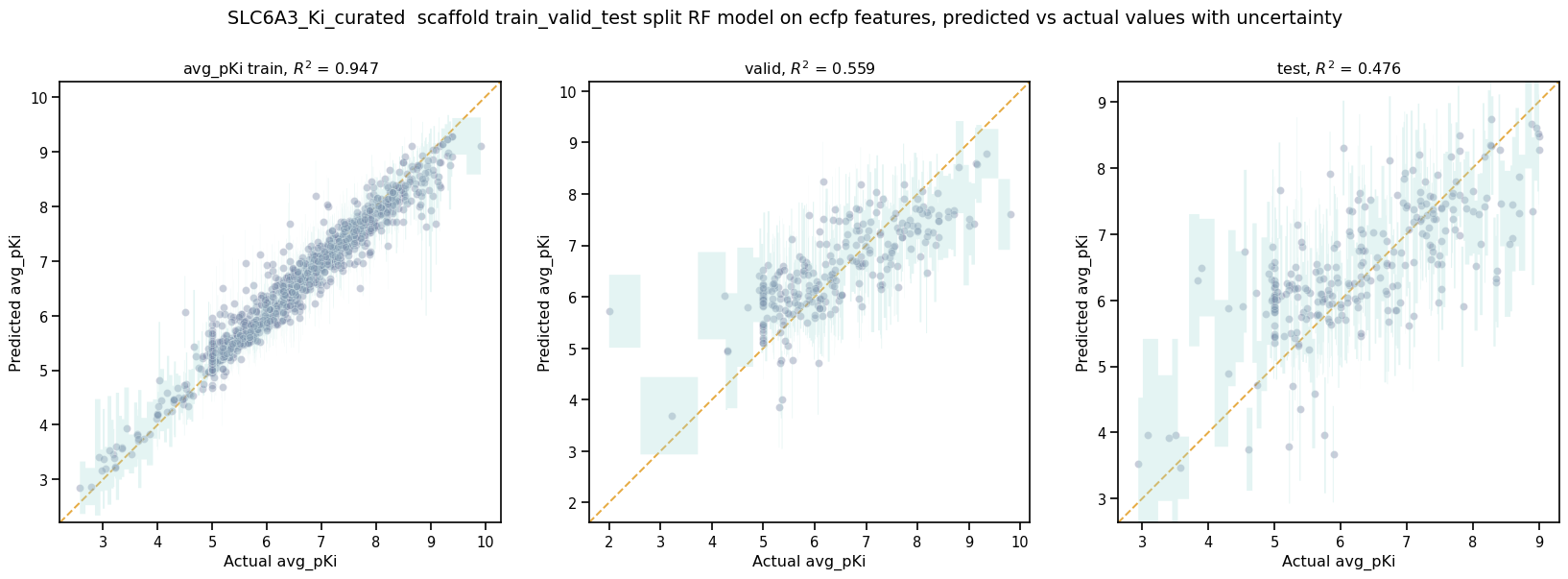
This RF model looks like it did better at training than the best NN model, even though its performance validation score is slightly lower. The low \(pKi\) values are learned more accurately in the training set, and the censored data at \(pKi\) =5 is also predicted more accurately.

# plot best xgboost model
model_type='xgboost'
model_path=result_df[result_df.model_type==model_type].iloc[0].model_path
pp.plot_pred_vs_actual_from_file(model_path)
print('\nBest valid r2 score: ',result_df[result_df.model_type==model_type].iloc[0].best_valid_r2_score)
print('\nModel Parameters: ',result_df[result_df.model_type==model_type].iloc[0].model_parameters_dict,'\n')

Best valid r2 score:  0.5031490908520113

Model Parameters:  {"xgb_colsample_bytree": 1.0, "xgb_gamma": 0.0019288871251215423, "xgb_learning_rate": 0.2158168689218416, "xgb_max_depth": 6, "xgb_min_child_weight": 1.0, "xgb_n_estimators": 100, "xgb_subsample": 1.0}

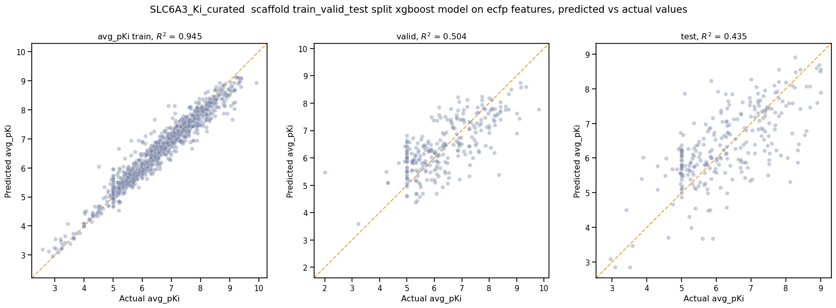
This XGBoost model learns the low \(pKi\) values better but still suffers from problems with predicting the censored data.

Moving forward, we would select the RF model as the best performer.

In Tutorial 7, “Train a Production Model”, we will use the best-performing parameters to create a production model for the entire dataset.

If you have specific feedback about a tutorial, please complete the AMPL Tutorial Evaluation.