04 Application of a Trained Model¶

Published: June, 2024, ATOM DDM Team

Please check out the companion tutorial video:

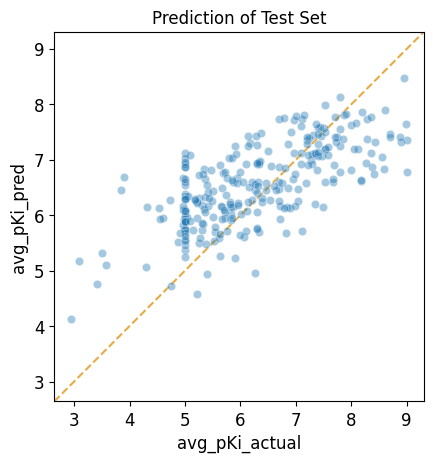
In this tutorial we will show you how to use a trained model to make predictions for a new set of compounds. As an example, we will take the model trained in “Tutorial 3: Train a Simple Regression Model”, which predicts \(pK_i\) values for inhibition of SLC6A3, and apply it to the test subset compounds from the original training dataset. Since we know the actual \(pK_i\) values for these compounds, we will then plot the predicted values against the actual values to see how well the model performs on this compound set.

This tutorial focuses on these AMPL functions:

import pandas as pd
import numpy as np
import matplotlib.pyplot as plt
import seaborn as sns

# ignore sklearn future warnings
import warnings
warnings.filterwarnings('ignore',category=FutureWarning)

from atomsci.ddm.pipeline import predict_from_model as pfm
from sklearn.metrics import r2_score

Creating The Test Dataset¶

First, create a test set by selecting the test data from the curated dataset. Here we are using the pre-featurized dataset to save time.

split_file_path = 'dataset/SLC6A3_Ki_curated_train_valid_test_scaffold_c35aeaab-910c-4dcf-8f9f-04b55179aa1a.csv'
curated_data_path = 'dataset/scaled_descriptors/SLC6A3_Ki_curated_with_rdkit_raw_descriptors.csv'

split_data = pd.read_csv(split_file_path)

curated_data = pd.read_csv(curated_data_path)

test_ids=split_data[split_data.subset == 'test'].cmpd_id.unique()
test_data = curated_data[curated_data.compound_id.isin(test_ids)]

# show most useful columns
test_data[['compound_id', 'base_rdkit_smiles', 'avg_pKi']].head()

	compound_id	base_rdkit_smiles	avg_pKi
3	CHEMBL17157	CC(C)(C)c1ccc(C(O)CCCN2CCC(C(O)(c3ccccc3)c3ccc…	6.692504
7	CHEMBL3321789	OC1(c2ccc(Cl)cc2)CC2CCC(C1)N2CCCOc1ccc(F)cc1	6.207608
13	CHEMBL595638	CN1C2CCC1[C@@H](C(=O)OCc1cn(CCOC(=O)[C@H]3C4CC…	7.795880
28	CHEMBL4447975	COc1cc(OC)c2c(c1)OC[C@@]1(C)NCC[C@@H]21	5.000000
41	CHEMBL1062	CC(=O)[C@@]1(O)CC[C@H]2[C@@H]3CCC4=CC(=O)CC[C@…	5.260744

Performing Predictions¶

Next, load a pretrained model from a model tarball file and run predictions on compounds in the test set. If the original model response_col was avg_pKi, the returned data frame will contain columns avg_pKi_actual, avg_pKi_pred, and avg_pKi_std. The predictions of \(pK_i\) are in the column, avg_pKi_pred. The avg_pKi_std column contains uncertainity estimates (standard deviations) for the predictions.

Here we set the is_featurized parameter to true, since we’re using the pre-featurized dataset.

Note

For the purposes of this tutorial, the following model has been altered to work on every file system. In general, to run a model that was trained on a different machine, you need to provide the path to the local copy of the training dataset as an additional parameter called “external_training_data”.

model_dir = 'dataset/SLC6A3_models/SLC6A3_Ki_curated_model_9ff5a924-ef49-407c-a4d4-868a1288a67e.tar.gz'
input_df = test_data
id_col = 'compound_id'
smiles_col = 'base_rdkit_smiles'
response_col = 'avg_pKi'

# loads a pretrained model from a model tarball file and runs predictions on
# compounds in an input data frame
pred_df = pfm.predict_from_model_file(model_path = model_dir,
                                      input_df = test_data,
                                      id_col = id_col ,
                                      smiles_col = smiles_col,
                                      response_col = response_col,
                                      is_featurized=True)


# show most useful columns
pred_df[['compound_id', 'base_rdkit_smiles', 'avg_pKi_actual','avg_pKi_pred', 'avg_pKi_std']].head()

Standardizing SMILES strings for 273 compounds.

	compound_id	base_rdkit_smiles	avg_pKi_actual	avg_pKi_pred	avg_pKi_std
0	CHEMBL17157	CC(C)(C)c1ccc(C(O)CCCN2CCC(C(O)(c3ccccc3)c3ccc…	6.692504	7.741641	1.289527
1	CHEMBL3321789	OC1(c2ccc(Cl)cc2)CC2CCC(C1)N2CCCOc1ccc(F)cc1	6.207608	6.607851	1.069817
2	CHEMBL595638	CN1C2CCC1[C@@H](C(=O)OCc1cn(CCOC(=O)[C@H]3C4CC…	7.795880	6.784137	1.271238
3	CHEMBL4447975	COc1cc(OC)c2c(c1)OC[C@@]1(C)NCC[C@@H]21	5.000000	6.080245	1.321997
4	CHEMBL1062	CC(=O)[C@@]1(O)CC[C@H]2[C@@H]3CCC4=CC(=O)CC[C@…	5.260744	6.304104	1.517846

Evaluating Prediction Performance¶

Then, calculate the \(R^2\) score and compare it with the expected test \(R^2\) score of 0.426594, reported in Tutorial 3, “Train a Simple Regression Model”.

actual_value = pred_df['avg_pKi_actual']
predicted_value = pred_df['avg_pKi_pred']
r2 = np.round(r2_score(actual_value, predicted_value), 6)
r2

0.426594

Visualizing Prediction Results¶

We can visualize the results in a scatter plot of predicted values vs. actual values.

from atomsci.ddm.pipeline import perf_plots as pp

# Plots predicted vs actual values from a trained regression model for a given
# dataframe
pp.plot_pred_vs_actual_from_df(pred_df,
                               actual_col='avg_pKi_actual',
                               pred_col='avg_pKi_pred',
                               label='Prediction of Test Set');

../_images/04_application_trained_model_10_0.png

In Tutorial 5, “Hyperparameter Optimization”, we will move beyond a single model and learn to optimize model hyperparameters by training many models.

If you have specific feedback about a tutorial, please complete the AMPL Tutorial Evaluation.